De-anonymizing the ATP 28

Overview

Last Sunday, Buzzfeed and the BBC published a joint investigation titled ‘The Tennis Racket’, which raised questions about whether a coterie of professional tennis stars have been fixing their own matches in exchange for payouts.

The article mentioned multiple groups of players:

A ‘core group of 16’:

The sport’s governing bodies have been warned repeatedly about a core group of 16 players – all of whom have ranked in the top 50 – but none have faced any sanctions and more than half of them will begin playing at the Australian Open on Monday.

‘15 players who regularly lost matches [with] heavily lopsided betting’:

BuzzFeed News began its investigation after devising an algorithm to analyse gambling on professional tennis matches over the past seven years. It identified 15 players who regularly lost matches in which heavily lopsided betting appeared to substantially shift the odds – a red flag for possible match-fixing.

28 players investigated by the Association of Tennis Professionals (ATP) for suspected match-fixing:

Nigel Willerton, who leads the Tennis Integrity Unit (TIU) set up to enforce fair play following the 2008 investigation, acknowledged that authorities had drawn a line under the evidence uncovered in the 2008 probe. The leaked files show that investigators implicated 28 players in suspected fixing and urged that they face a full disciplinary investigation. But Willerton said that tennis authorities took no action against them.

Buzzfeed learned about both the first and last of those three groups via leaked documents. The second group, containing 15 players, was unearthed by Buzzfeed’s own investigation into suspicious betting patterns:

The investigation into men’s tennis by BuzzFeed News and the BBC is based on a cache of leaked documents from inside the sport – the Fixing Files – as well as an original analysis of the betting activity on 26,000 matches and interviews across three continents with gambling and match-fixing experts, tennis officials, and players.

However, Buzzfeed’s article anonymized the names of the players in all three groups:

BuzzFeed News and the BBC have chosen not to name the players whose matches have repeatedly been flagged for attracting highly suspicious betting, because without access to phone, bank, or computer records it is not possible to prove a link between the players and the gamblers.

Nevertheless, the Buzzfeed 15 (as they have been dubbed) have already been successfully de-anonymized by multiple sources via a reconstruction of BuzzFeed’s methodology.

Moreover, and this is a very important point, serious doubts have been raised (both in the Buzzfeed article itself, as well as by third parties) as to whether the betting patterns of the Buzzfeed 15 indicate evidence of match-fixing at all. At the very least, it is clear that the presence of a player’s name on that list is not equivalent to being suspected of match-fixing, especially without corroborating evidence.

For that matter, the same principle applies both to the core group of 16, as well as the 28 players named in the 2008 report: without additional context, it is difficult or even impossible for the general public to draw meaningful conclusions about match-fixing from names on a list.

In any case, this leaves two groups that are still (to my knowledge) anonymized. The first group, the ‘core group of 16’, has not been publicly identified and probably won’t be for some time, if ever. This is because this group is sourced from a cache of leaked documents: if these documents never become public, it’s difficult to imagine how anyone will discover who the 16 players are with any degree of certainty.

However, it’s the list of 28 players that were investigated by the ATP back in 2008 (a process that eventually led to the creation of the sport’s anti-corruption body, the Tennis Integrity Unit) that drew my interest. Unlike the Buzzfeed report, which explicitly warned that its evidence was not sufficient to accuse the 15 players of match-fixing, the investigators recruited by tennis authorities in 2008 were former members of the British Horseracing Authority who were selected precisely because of their extensive experience researching gambling corruption.

For whatever reason, Buzzfeed included the hashed IDs of those 28 investigated players in their documentation. Strangely, the vast majority of the reaction to the Buzzfeed piece has focused disproportionately on the Buzzfeed 15: I have yet to see any attempt to reconstruct the original ATP 28.

What follows is my attempt to unearth those names. Please note that there are likely dozens of ways to arrive at a similar result. I chose to work almost entirely in Excel, but more tech-savvy folks are likely to use scripts (as in the Buzzfeed repository example) instead.

Methodology

Organizing the Buzzfeed dataset

The first order of business is to organize the Buzzfeed dataset in a way that allows us to easily match up anonymized player IDs with their win-loss records for each year.

Download the Buzzfeed dataset.
Open the file in Excel, and hit Data > Remove Duplicates, selecting only the checkbox for column P: ‘match_uid’. 26,533 rows remain, including the header row.
Create a pivot table from the dataset with the following settings:

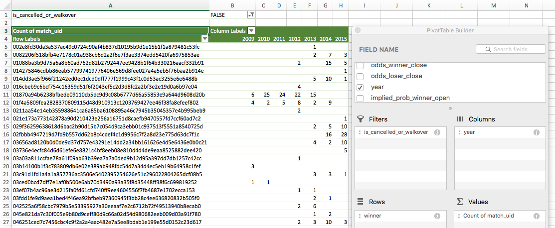
Note that ‘is_cancelled_or_walkover’ is filtered to only return rows with ‘FALSE’.
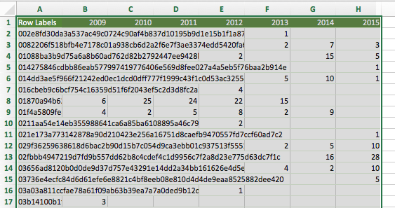
Copy the pivot table data (including header row, but excluding grand totals row) into a new worksheet:
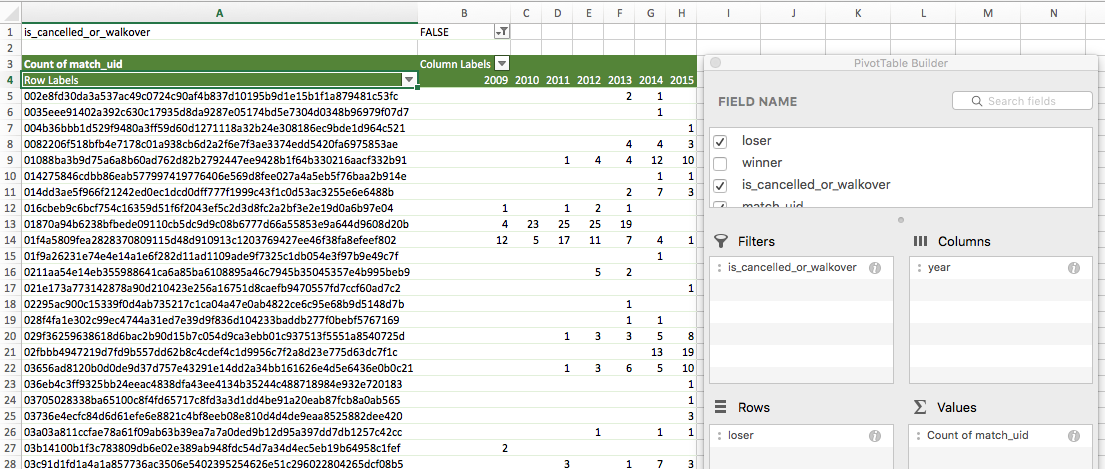
Return to the pivot table worksheet and replace ‘winner’ with ‘loser’ in the ‘Rows’ section of the PivotTable Builder:
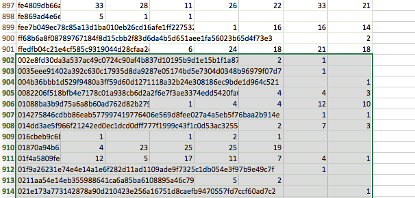
Copy the pivot table data (excluding both header row and grand totals row this time) to the other worksheet, just below the last row of your previously copied ‘winner’ data:
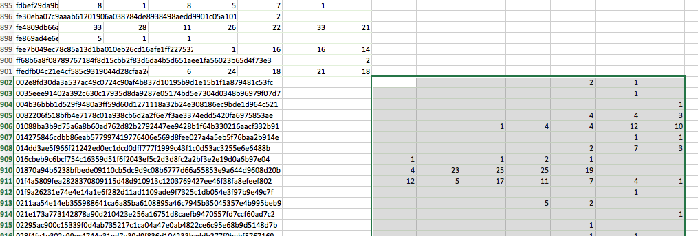
For the new ‘loser’ rows just copied over, move all columns except for the first one (column A, which contains the loser player IDs) to the right, so the leftmost column is one column to the right of all the ‘winner’ columns above:
Go back to the top and copy over the group of year column headers to the right, so there are two consecutive groups of columns for the years 2009-2015. Prefix the first group with ‘W’ for ‘winner’ and the second group with ‘L’ for ‘loser’:
Copy the list of 28 anonymized players named in the TIU report from the Buzzfeed GitHub repository to a new worksheet. In Excel, hit Edit > Find > Replace, and run Replace All (separately) on the ', [space], and , characters to replace them with empty text: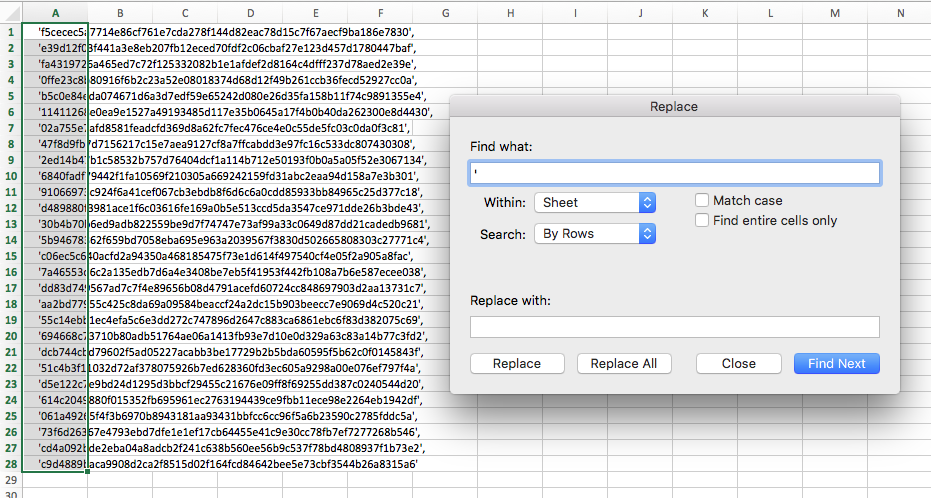
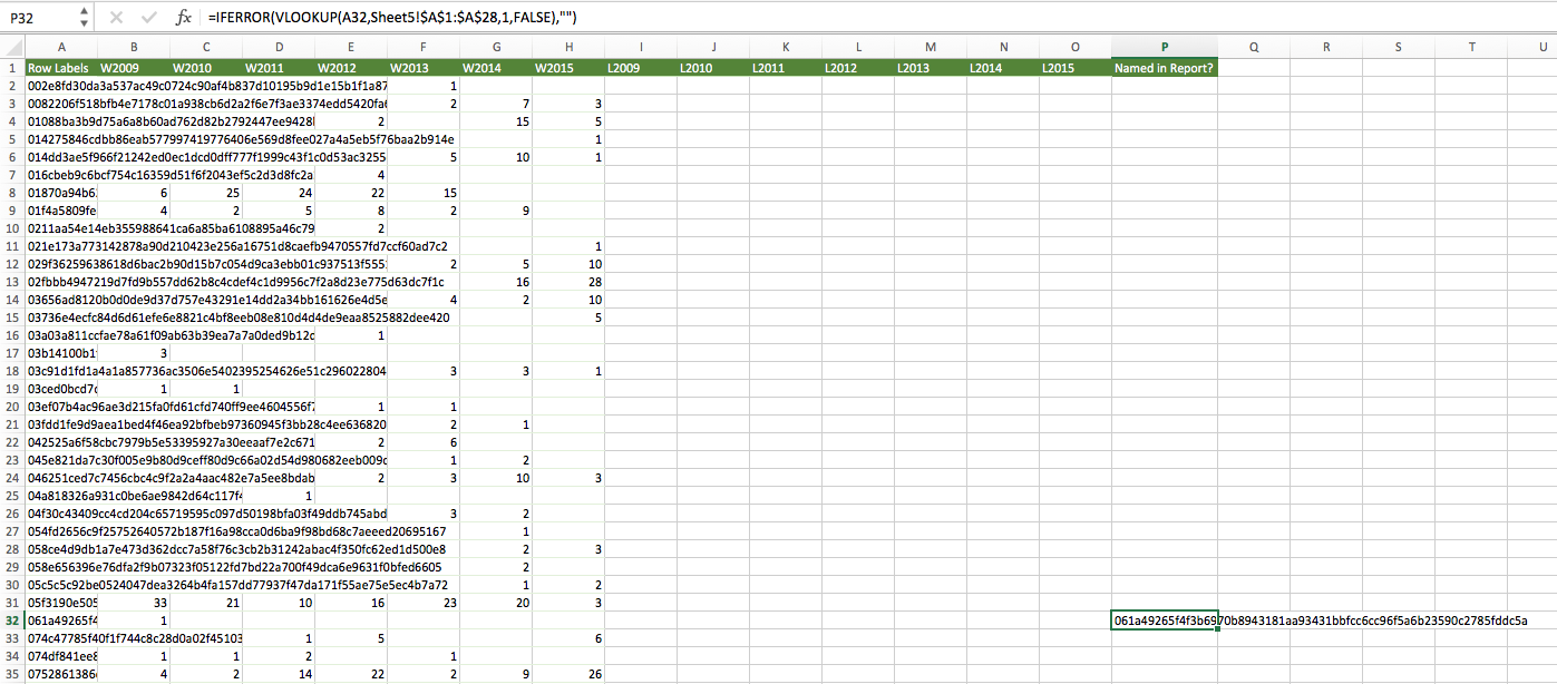
Go back to the worksheet from step 8 and add another column, column P, to the right of all the existing ones, called ‘Named in Report?’ Then enter the following formula in cell P2:
```
=iferror(vlookup(A2,Sheet5!$A$1:$A$28,1,false),"")
```
Be sure to change ‘Sheet5’ (if necessary) to whichever sheet holds the 28 anonymized IDs from the prior step. This formula copies the anonymized ID to the cell if it matches the current row, and leaves it blank if not.

Finally, apply this formula (by dragging or copy/pasting) to column P for all rows. Make sure the first part, ‘A2’, increases (to ‘A3’, ‘A4’, etc.) as the row numbers increase. The formula’s reference to the other sheet that contains the 28 IDs, however, should not increase:
Select all data (columns A through P, and all rows) and create a new pivot table with the following settings:

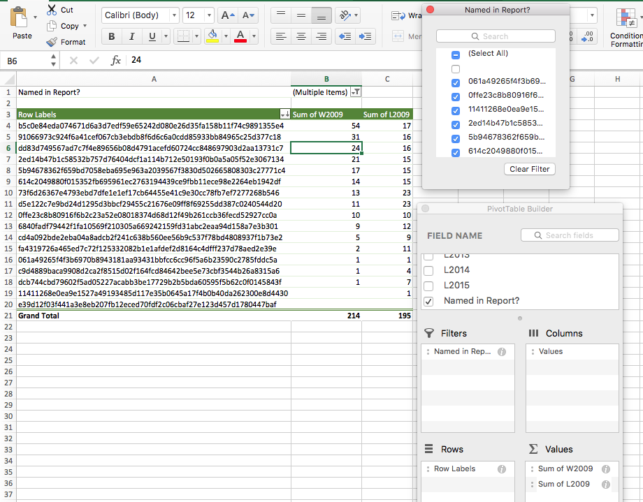
Note that the ‘Values’ section of the PivotTable Builder has been set to sums, not counts. I’ve also sorted the pivot table by wins, from most to least. Most importantly, I’ve included ‘Named in Report?’ to the ‘Filters’ section of the PivotTable Builder and unchecked the box for blank rows, which filters out all players who weren’t named in the 2008 report. I now have a table of anonymized players who were named in the report, sorted by wins for the year 2009.
Now add in all the other ‘W’ and ‘L’ year pairs, so the pivot table looks like this:

Organizing the historical match dataset

Clone the ‘tennis_atp’ GitHub repository (a terrific historical tennis dataset from Jeff Sackmann) to your local drive.
The repository contains many data files. Start by opening the one titled ‘atp_matches_qual_chall_2009.csv’, which contains ‘tour-level qualifying and challenger main-draw matches’ for 2009. Insert a new column to the left of the leftmost one (‘tourney_id’) and call it ‘year’ in cell A1. In the first data cell in that column (cell A2), type ‘2009’, then click and drag (or copy/paste) that value all the way down the column. Make sure it copies ‘2009’ and doesn’t increment it.
Next, open ‘atp_matches_qual_chall_2010.csv’. Copy all rows (except the header row) to the bottom of the ‘atp_matches_qual_chall_2009.csv’ file, just below the last row. Be sure the leftmost column of the copied data lines up with column B now, to match up the column data from both years. Then find the topmost row of the data you just copied over, type ‘2010’ in column A, and drag down again. Repeat this process for all years through 2015.
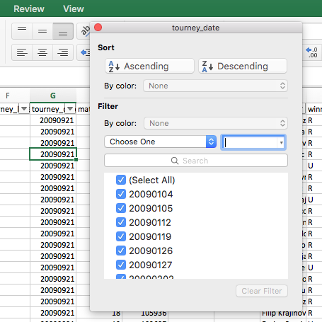
In Excel, hit Sort & Filter > Filter, then select the ‘tourney_date’ header and de-select all dates after September 24, 2015 (to match the Buzzfeed data, as explained by John Templon):
Select the entire filtered table, including header row, and copy it to a new sheet. Then delete the original sheet so only the new sheet remains, with all matches from the start of 2009 through September 24, 2015.
Open the file ‘atp_matches_2009.csv’ and repeat steps 2 through 5 with the data from that series of files: ‘atp_matches_2009.csv’, ‘atp_matches_2010.csv’, and so on. Those files contain ‘tour-level main draw matches’ and should be aggregated in exactly the same way as you’ve already done for the qualifying and challenger match data. Be sure to remove the rows for tourneys after September 24, 2009.
At this point you should have two files with aggregated data: one with qualifying and challenger matches and one with main draw matches. Now join them together, by copying and pasting the entire qualifying and challenger dataset directly below the main-draw one (minus the header row, since there’s already one at the top of the file you’re copying into).
You should now have a file containing 64,963 rows (including the header row) of all relevant matches from the start of 2009 through September 24, 2009. Create a pivot table of all of this data on a new sheet, using the following settings:

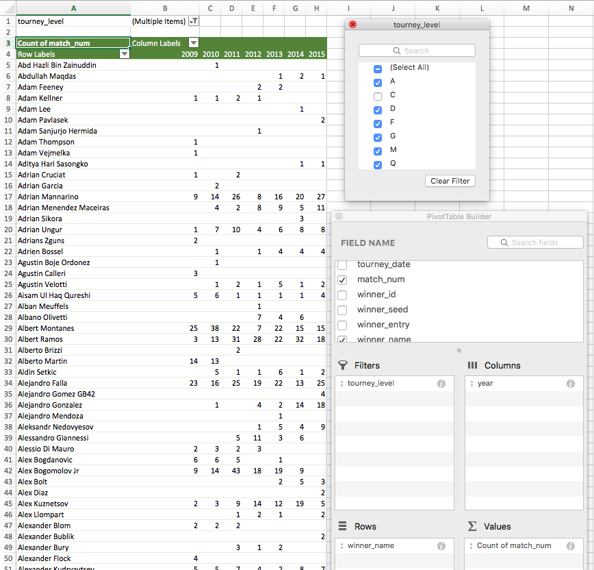
Notice a few things. First, ‘tourney_level’ is selected as a filter and the box for ‘C’ (meaning ‘Challenger’) is unchecked. This is because, in order to match Buzzfeed’s data, we do not want to include Challenger matches in this analysis. We’ve also made sure the ‘Values’ section of the PivotTable Builder is set to a count, not a sum, as we’re trying to obtain the count of wins by player.
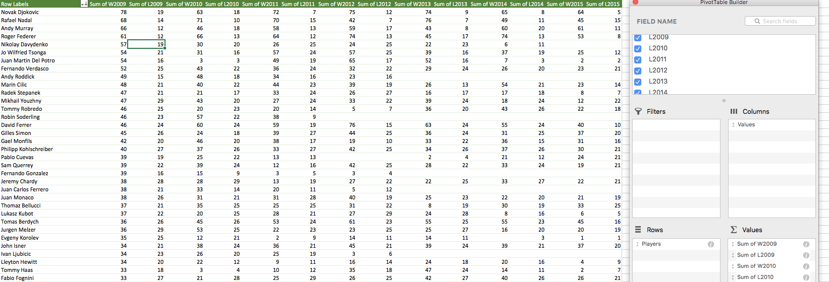
At this point we just need to replicate steps 4-8 of the ‘Organizing the Buzzfeed dataset’ section (but with the aggregated data from this section instead). Once this is complete, set up the new pivot table you’ve just created in those steps to include columns for wins and losses from each year, just as you did in the original Buzzfeed dataset. It should look something like this:

Matching up the two datasets

There are now two files. One contains a pivot table of the anonymized IDs from the 2008 report, along with their W-L records from 2009-2015. We’ll call this the ‘Buzzfeed data’. The other file contains a pivot table with the same columns, but attached to real player names from that period. We’ll call that the ‘ATP data’. What we need to do now is figure out which of those players from the ATP data match up with the anonymized IDs within the Buzzfeed data.

Keep in mind that, in many cases, the data won’t match up precisely, as Buzzfeed used odds data to assemble their dataset. So any matches that didn’t have odds from their selected bookmakers won’t be present. In order to deal with these discrepancies, I’m stealing a page from the Show Legend playbook and will be using root mean square error (RMSE) to find the closest matches.

Let’s begin by copying over the data from each of the pivot tables from those two files into separate worksheets within the same new workbook. Make sure to include the header row and table data, but not the grand total row at the bottom. The copied data should not be a pivot table, but it should include the same data. Here, for example, is how the anonymized IDs worksheet should roughly look:
Notice that the Buzzfeed data only includes 17 IDs, not 28. This is because only 17 of the 28 players named in the 2008 ATP report played in any of the roughly 26,000 matches Buzzfeed selected from OddsPortal.com. For each of these 17 IDs, we’re going to calculate the RMSE for each season’s wins and losses as compared to all 2,328 named players in the ATP data.

Just as an example, say we’re trying to figure out the identity of ID 5b94678362f659bd7058eba695e963a2039567f3830d502665808303c27771c4. That player won 7 and lost 10 matches in 2014. If we were comparing that ID to, say, Nikolay Davydenko for the same year (he went 6-11), we’d first calculate the difference between the two players’ wins (7 - 6 = 1) and losses (10 - 11 = -1). Then we’d square both values (1^2 = 1, and -1^2 = 1) and calculate the average of the squared errors: 1 + 1 = 2, divided by 2 observations (2014 wins, and 2014 losses), which is 1. The square root of 1 is 1, so that’s the root mean square error (RMSE) in this example.

In reality, though, we’re not interested in comparing player-seasons: we want to compare players overall. That is, we want to know the identity of the anonymized IDs, not specific seasons they had. So we’re not only going to look at the 2014 wins and losses, but also 2013, 2012, etc. for all 7 seasons of data we’re comparing (2009-2015).

To do this, for each anonymized ID, we have to iterate through every single player in the ATP data and compare all 14 observations for each player (wins and losses for each of the 7 years) with the same data from the anonymized player. We then sum the squares of every difference between the two (2009 wins vs. 2009 wins, 2009 losses vs. 2009 losses, 2010 wins vs. 2010 wins, etc.), average them (we do this by dividing by 14, which is the total number of observations), and finally find the square root.

Once we’ve done these thousands of calculations (17 anonymized IDs x 2,328 named players = 39,576 RMSEs), we can sort all 2,328 players from lowest to highest RMSE for each anonymized ID, in order to find the closest matches between anonymized and named players. A low RMSE will indicate that the year-by-year wins and losses for the anonymized ID match up closely with the year-by-year wins and losses for a given named player. This is a lot of calculations across all IDs and players, but they can be easily executed using Excel formulas.
The first thing we need to do is eliminate several of the 17 anonymized IDs due to lack of data. Take a look at the data for the following IDs:
```
 061a49265f4f3b6970b8943181aa93431bbfcc6cc96f5a6b23590c2785fddc5a
 11411268e0ea9e1527a49193485d117e35b0645a17f4b0b40da262300e8d4430
 dcb744cbd79602f5ad05227acabb3be17729b2b5bda60595f5b62c0f0145843f
 e39d12f03f441a3e8eb207fb12eced70fdf2c06cbaf27e123d457d1780447baf
 fa4319726a465ed7c72f125332082b1e1afdef2d8164c4dfff237d78aed2e39e
 73f6d26367e4793ebd7dfe1e1ef17cb64455e41c9e30cc78fb7ef7277268b546
 cd4a092bde2eba04a8adcb2f241c638b560ee56b9c537f78bd4808937f1b73e2
```
All 7 of the above cases have very little data: either they only have data from 1 of the 7 seasons we’re analyzing, or their data across multiple seasons is too sparse to compare meaningfully with named players. So we’re going to exclude them from our analysis, leaving only 10 anonymized IDs.

Now, on the worksheet with ATP data, we’ll want to add new column headers (to the right of the named players’ win-loss data) for each of the 10 IDs. It will look something like this:

Now, here’s the Excel formula I used to calculate the root mean square error (in cell P2 in the above screenshot):
```
 =SQRT(((VALUE($B2)-VALUE(VLOOKUP(P$1,'Buzzfeed Data'!$A$2:$O$18,2,FALSE)))^2+(VALUE($C2)-VALUE(VLOOKUP(P$1,'Buzzfeed Data'!$A$2:$O$18,3,FALSE)))^2+(VALUE($D2)-VALUE(VLOOKUP(P$1,'Buzzfeed Data'!$A$2:$O$18,4,FALSE)))^2+(VALUE($E2)-VALUE(VLOOKUP(P$1,'Buzzfeed Data'!$A$2:$O$18,5,FALSE)))^2+(VALUE($F2)-VALUE(VLOOKUP(P$1,'Buzzfeed Data'!$A$2:$O$18,6,FALSE)))^2+(VALUE($G2)-VALUE(VLOOKUP(P$1,'Buzzfeed Data'!$A$2:$O$18,7,FALSE)))^2+(VALUE($H2)-VALUE(VLOOKUP(P$1,'Buzzfeed Data'!$A$2:$O$18,8,FALSE)))^2+(VALUE($I2)-VALUE(VLOOKUP(P$1,'Buzzfeed Data'!$A$2:$O$18,9,FALSE)))^2+(VALUE($J2)-VALUE(VLOOKUP(P$1,'Buzzfeed Data'!$A$2:$O$18,10,FALSE)))^2+(VALUE($K2)-VALUE(VLOOKUP(P$1,'Buzzfeed Data'!$A$2:$O$18,11,FALSE)))^2+(VALUE($L2)-VALUE(VLOOKUP(P$1,'Buzzfeed Data'!$A$2:$O$18,12,FALSE)))^2+(VALUE($M2)-VALUE(VLOOKUP(P$1,'Buzzfeed Data'!$A$2:$O$18,13,FALSE)))^2+(VALUE($N2)-VALUE(VLOOKUP(P$1,'Buzzfeed Data'!$A$2:$O$18,14,FALSE)))^2+(VALUE($O2)-VALUE(VLOOKUP(P$1,'Buzzfeed Data'!$A$2:$O$18,15,FALSE)))^2) / 14)
```
That formula looks scarier than it is. In reality, it just calculates the difference between each of the 14 observations for each named player (wins and losses from each of the 7 seasons we’re analyzing) and the anonymized player named in that particular column header (P1, in this case). The VLOOKUPs simply find the corresponding win and loss data from the worksheet tab with the Buzzfeed (anonymized) data. Of course, you may have to modify this formula to fit your worksheets depending on your naming conventions and so on.

I constructed the formula to be draggable: that is, you can drag both rightward (to analyze other anonymized IDs) and downward (to analyze other named players). This will quickly generate thousands of RMSE calculations on the spot (although it will be fewer than the 39,576 mentioned above, because we’ve eliminated 7 IDs from the comparison):

The last step is just to select all of those newly calculated cells, copy them, and then use Edit > Paste Special to paste them as values in the same place. This gets rids of the formulas and replaces them with actual numbers. Once this is complete, you can use the Sort & Filter command on any of the 10 anonymized ID columns in order to sort from smallest to largest RMSE. You now have the best guesses for who these anonymized IDs actually are. Below is the list of 10, along with the three closest guesses (RMSE value in parentheses):

Anonymous ID	Closest Guess	2nd Guess	3rd Guess
2ed14b47b1c58532b757d76404dcf1a114b712e50193f0b0a5a05f52e3067134	Richard Gasquet (1.41)	John Isner (5.75)	Stanislas Wawrinka (5.78)
0ffe23c8b80916f6b2c23a52e08018374d68d12f49b261ccb36fecd52927cc0a	Juan Ignacio Chela (3.06)	Ryan Sweeting (4.77)	Peter Luczak (5.94)
5b94678362f659bd7058eba695e963a2039567f3830d502665808303c27771c4	Michael Llodra (1.89)	Olivier Rochus (5.06)	Bjorn Phau (5.24)
614c2049880f015352fb695961ec2763194439ce9fbb11ece98e2264eb1942df	Dmitry Tursunov (2.42)	Daniel Brands (6.32)	Blaz Kavcic (8.17)
6840fadf79442f1fa10569f210305a669242159fd31abc2eaa94d158a7e3b301	Maximo Gonzalez (2.07)	Alexander Kudryavtsev (4.08)	Jesse Huta Galung (4.22)
91066973c924f6a41cef067cb3ebdb8f6d6c6a0cdd85933bb84965c25d377c18	Fernando Gonzalez (2.22)	Alexander Peya (3.51)	Sebastien De Chaunac (4.15)
b5c0e84eda074671d6a3d7edf59e65242d080e26d35fa158b11f74c9891355e4	Nikolay Davydenko (1.34)	Radek Stepanek (6.39)	Lukasz Kubot (6.66)
c9d4889baca9908d2ca2f8515d02f164fcd84642bee5e73cbf3544b26a8315a6	Filippo Volandri (2.60)	Adrian Ungur (5.55)	Rogerio Dutra Silva (5.93)
d5e122c7e9bd24d1295d3bbcf29455c21676e09ff8f69255dd387c0240544d20	Potito Starace (3.17)	Philipp Petzschner (5.62)	Igor Kunitsyn (5.69)
dd83d749567ad7c7f4e89656b08d4791acefd60724cc848697903d2aa13731c7	Albert Montanes (1.51)	Somdev Devvarman (5.29)	Daniel Gimeno Traver (6.55)

So what are we looking at here? Well, to take the first example, the best guess is Richard Gasquet, with a root mean square error of 1.41. Let’s take a look at his W-L record against ID 2ed14b47b1c58532b757d76404dcf1a114b712e50193f0b0a5a05f52e3067134:

Year	Anonymous Player W-L	Richard Gasquet W-L
2009	21-15	24-16
2010	38-22	38-24
2011	34-19	35-20
2012	45-23	42-22
2013	49-23	50-23
2014	31-19	31-20
2015	34-12	34-12

As you can see, these records match up quite closely. Take a look at 2009: the anonymized player went 21-15, while Gasquet went 24-16. That’s a difference of 3 wins and 1 loss. Each of those differences must be squared: so 3 becomes 9, and 1 stays 1. And so on for each year. The sum of all squared errors here is 28, divided by 14 observations. This leaves a quotient of 2, and the square root of that is 1.41 – the root mean square error.

Final thoughts

Important dataset caveats

It’s worth noting that, since Buzzfeed only released an anonymized version of the OddsPortal data they used, I had to compare that anonymized dataset with a completely separate one (the Jeff Sackmann repository). This necessarily introduces discrepancies and reduces accuracy – especially given Buzzfeed’s methodology, which only counted matches with odds from specific bookmakers.

Along the same vein, the RMSE is heavily skewed for players with little data. This is why I eliminated 7 IDs right off the bat: with so little data, the RMSE is artificially low because no errors are counted in years when data doesn’t exist for both the player and the anonymized ID. That doesn’t necessarily mean that the match is incorrect: it’s possible the player and the anonymized ID are in fact the same person, and he simply didn’t play in any of those years in which we have no data. But without further investigation it’s difficult to know for certain, so I’ve excluded them out of caution.

Finally, this almost goes without saying, but the above list represents players who are possibly named in the 2008 ATP report, based on their W-L records. It does not constitute proof that they are actually guilty of match-fixing. Indeed, it doesn’t even prove that they’re in the report – although in certain cases, like Richard Gasquet, Albert Montanes, and so on, it appears highly likely. All of this, of course, assumes Buzzfeed correctly identified the players in the report. It would be surprising if that were not the case (since the names were leaked to them), but it’s worth mentioning.

Anonymity is the new fame

I can’t help but conclude that Buzzfeed intentionally made it as easy as possible to de-anonymize these players’ names. This goes not only for the Buzzfeed 15, whose IDs have already been de-anonymized by others, but also for any of the IDs in their ‘aggregated_betting_data.csv’ dataset generally.

Just to take a simple example, a cursory examination of the Buzzfeed data (using the methodology described above under ‘Organizing the Buzzfeed dataset’) reveals that the player 797e56532b5b820177672d897d38dc7017979199a24ceba1497c89ea9c318cfe had the most wins of any player in 2014, with 73 victories against 12 losses.

A quick visit to CoreTennis.net reveals that Roger Federer had exactly that record in 2014.

In that same year, player 4c1fa9086ee7dd8663600a9365fbc4193931c5533ca489aa9fcd17724c6b5dac went 61-8. According to CoreTennis.net, this record is identical to that of Novak Djokovic. (To be perfectly clear, neither of these player IDs was on the Buzzfeed 15 nor the ATP 28, and there is no reason to suspect they were in the ‘core group of 16’ obtained by Buzzfeed either.)

Why would they do this? One possible explanation is that, in partnering with the BBC on this investigation, both organizations were subject to the United Kingdom’s more stringent libel laws. (As a non-lawyer, I have no idea how, or if, the UK’s laws would apply to Buzzfeed on a joint investigation.) In such a case, Buzzfeed’s attorneys may have argued against naming the players, but that wouldn’t necessarily prevent Buzzfeed from making it extraordinarily easy for the general public to uncover them.

A related, but far less likely, possibility is that Buzzfeed initially intended to publish the names but was barred due to a super-injunction in the UK, preventing them not only from publishing the names but also from revealing that they were prohibited to do so. (There is some precedent for actions such as this. Again, I have no idea if this would apply to an American news organization partnering with a British one, however.)

Feedback

Having trouble replicating my results? Does something not make sense? Is there an error in my methodology? Let me know in the comments, or on Twitter.